The DU IRMIA++ students' journal - ITI IRMIA++ - Research in Mathematics, Interactions & Applications

This page presents a collection of articles written by the DU IRMIA++ students and based on the interdisciplinary seminar.

Page contents

16/11/2023 - Visualization and algebraic geometry

This article was written by Ludovic FELDER and Ruben VELKY, based on the presentations given by Laurent BUSÉ and Jean-Michel DISCHLER on November 16th, 2023

Artists started giving their paintings an impression of 3D a couple hundred years ago, in order to make them realistic. The principle is pretty easy : combining a 2D support with colors and a perspective representation to give the illusion of a 3D scene. Computer generated images use the same principle except that the image isn’t on a canvas but on a screen. Since the first real time computers in the 1950’s, a lot of work regarding image generation has been done. One crucial invention to get realistic images is ray-tracing.

Ray-tracing is a technique used to model the transport of light through a 3D scene in order to generate a digital image. All we need are three elements : a light sources, objects and sensors. Light propagates from the source, then is reflected or absorbed by the objects before eventually reaching the sensors, that is the plane surface that generates the image. As an approximation, light behaves like rays that propagate in straight lines and carry an energy distribution for each wave length, called radiance. The interaction between light and an object is modelled using the so-called bidirectional reflection distribution function (BRDF), which contains all the information regarding the material of the object and its micro structure. To get a full image of a 3D scene, we therefore need to determine all the light rays reaching each pixel. In practice, we use a Monte-Carlo techniques to sample a few rays per pixel and compute the accumulated radiance. Unlike the direct light from the source to the sensors, the indirect light which undergoes several reflections before reaching the pixels is quite computationally demanding and the results may be quite noisy.

Figure 1. Images generated by metropolis light transport (Source: [1])

Many techniques have been developed to generate better images in shorter time. For instance, as many rays actually carry a low level of radiance, importance sampling is used to select the rays directions according to the radiance distribution. This can be done adaptively based on the radiances previously calculated. One key point in the ray tracing algorithms concerns the intersection computation between the rays and the objects. To speed up the computations, the objects can be enclosed into bounding volumes to quickly check whether the rays reach the object or not.

We are now going to introduce more specific techniques for problems involving the intersection between a ray and the surface of an object or, more generally, between two objects. Here we are particularly interested in the case where the surface of the object is parameterized by rational fractions, that are fractions between two polynomials. Indeed, we will see how algebraic geometry tools can be used to tackle intersection problems and solve real-life problems, like manufacturing objects of a given shape.

Suppose that the contour of a two-dimensional object is represented by two parametrized curves, finding the intersection points of these two curves can be a crucial step in programming the milling machine that will carve the object. The method used to find their intersection points relies on the Sylvester resultant, which is the determinant of a matrix in the coefficients of the rational fractions defining a parametrized curve. The Sylvester resultant provides an implicit equation for one curve. After inserting the parametrization of the second curve into this implicit equation, we get a polynomial equation to find out the intersection points. The whole problem can actually be reformulated as a generalized eigenvalue problem and therefore efficient numerical linear algebra methods can be used to make the computations.

The extension to the intersection between a curve and a surface is more intricate. One difficulty comes from the base points of the surface, which are points for which the parameterization is not well defined projectively. To overcome this difficulty, instead of resultant-based methods, a non square matrix, called matrix of syzygies, is considered : its rank drops out exactly on the surface. Then plugging the parameterization of the curve gives us a univariate polynomial matrix. As before, the drop in rank of this matrix can be reformulated as a generalized eigenvalue problem.

These problems are good examples of how algebraic geometry can be used in concrete cases. While seeming quite simple, these problems require in fact some advanced theory, especially for complex geometrical shapes.

References:

[1] Veach E., Guibas L. J. (1997). Metropolis light transport. Proceedings of the 24th annual conference on Computer graphics and interactive techniques.

09/11/2023 - Equilibria in astrophysics and fluid dynamics

This article was written by Vishrut BEZBARUA and Hans Joans ZEBALLOS RIVERA, based on the presentations given by Hubert BATY and Victor MICHEL-DANSAC on November 9th, 2023.

This article discusses the challenges of simulating fluid flows around equilibrium states, from the sun’s corona to river currents. We’ll also highlight innovative computational strategies for greater precision.

Solar flares are sudden and intense explosions in the solar corona, involving the release of magnetic energy stored in the Sun’s atmosphere. They are sudden and fast, releasing energy equivalent to 10²⁵ times that of the Hiroshima Bomb. Ejected flows have speeds close to 0.01 times the speed of light, and the strongly accelerated particles acquire relativistic speeds. There are energy releases along with the solar flares, which finds its origin in magnetic processes, a prominent example of which is magnetic reconnection. Magnetic reconnection is a fundamental process where the magnetic topology undergoes a sudden rearrangement, converting magnetic energy into kinetic energy, thermal energy, and particle acceleration. This process occurs when magnetic field lines with opposing orientations come into close proximity, leading to the breaking and reconnecting of these field lines and formation of structures called plasmoids which are like self-contained plasma fluid quantities.

To study the dynamics of these plamoids, the complete set of the so-called magnetohydrodynamic (MHD) equations have to be solved: this is a highly intricate task. Numerical methods have to be carefully chosen in order to treat both conservation and diffusive parts of the equations. To simplify the computational challenges associated with solving the MHD equations in such physical regime, researchers often employ reduced models, particularly in two dimensions. In such simplified models, certain complexities inherent in the plasmoid regime can be mitigated, offering advantages in terms of computational efficiency.

Figure 1. A finite element discretization

To perform numerical simulations of such models, a common approach is to consider a finite-element method, which provides a piece-wise polynomial approximation of the physical quantity. This method can be used for a detailed numerical study of magnetic reconnection and tilt instability. In the regime where the Lundquist number exceeds 10⁴, stochastic reconnection, characterized by the presence of numerous plasmoid, becomes prominent. However, problems arise because the number of elements and the calculation time required then increase considerably. The computational limit is reached for a Lundquist number of the order of 10⁶.

Recently, a cheaper alternative has been proposed using a Physics-Informed Neural Network (PINN) approach, which is proving effective for two-dimensional MHD equilibria. PINNs consist in finding out a solution represented by a neural network, whose parameters are optimized to satisfy the physical model at some sampling points. They offer a mesh-free solution without complex discretization. Despite merits, challenges include the non-convex optimization of the parameters and limited extrapolation. Ongoing efforts aim to refine training methodologies, highlighting PINNs’ promise in diverse applications.

Exploring equilibrium states in astrophysics, such as plasmoids in solar flares using MHD models, alongside AI-enhanced resolution through techniques like PINNs, provides valuable insights into the stability of complex systems. Shifting focus to fluid mechanics, we examine the numerical techniques developed for simulating shallow water flows. Like MHD equations, many fluid models actually describe conservation laws (conservation of mass, momentum, energy): they belong to the class of the so-called hyperbolic equations. Specific numerical methods, called Finite Volume Method, have been developed topreserve these conservation laws at the discrete level. This approach becomes crucial in situations where physical phenomena can generate discontinuities or singularities in the solutions. For instance, these methods were used for numerical simulations of the Saint Venant model, which model tsunamis, or a section of the Gironde estuary (see Figure 2).

The Saint-Venant equations provides the dynamics of the height of water h(x,t) above a topographic level z(x,t) and the volumetric flux q(x,t). In the 1D case, the equations are the following partial differential equations:

where g is the gravity constant and η = 7/3 is the Manning coefficient, which characterizes the friction with the ground level. This system is indeed a hyperbolic system with source term, which can be written under the general form:

with W(x,t)=(h(x,t),q(x,t)). To discretize such a system with a Finite Volume Scheme, the one-dimensional domain between the border points a and b is subdivided into N subintervals:

Then, the scheme is inspired from the following integral formulation of the conservations laws obtained after the integration of the equation over the cell [x_i−1/2,x_i+1/2] between time tⁿand tⁿ⁺¹:

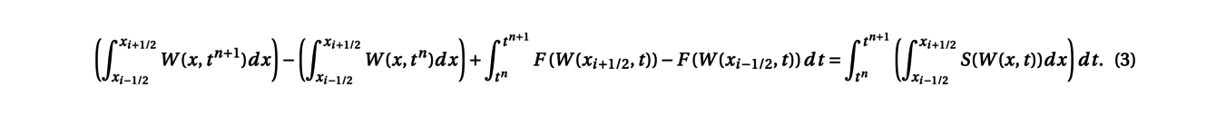
Denoting by W_iⁿan approximation of the average of the solution W(x,t) over the cell [x_i−1/2,x_i+1/2] at time tⁿ, a finite volume scheme thus writes:

where the function F is the numerical flux function and S the numerical source term. In the absence of a term source, such a discretization preserves the total quantity over the domain:

When solving the Saint-Venant system, a key property is to ensure that the method is well-balanced, meaning that it exactly preserves the discrete steady-state solutions. One particular steady state is the lake at rest, with zero flux q = 0 and constant level of the lake, h + z = constant. Such property is crucial to avoid the generation of artificial errors and a classical method for the lake at rest steady state is the so-called hydrostatic recontruction. The function F and S have to be defined such as to satisfy W_iⁿ⁺¹ = W_iⁿwhen starting from a steady state. Recent developments have also made it possible to take moving steady states (with q≠ 0) into account.

In conclusion, whether for the simulation of magnetic reconnection or shallow water fluid mechanics, very elaborate and efficient numerical resolution tools have been studied to faithfully capture either the dynamics around equilibria. Exact preservation of steady states can be prescribed into the numerical method, while new machine learning tools can help to overcome numerical constraints and tackle extended physical regimes.

05-19/10/2023 - Kirkman’s problem and statistical design of experiments

This article was written by Abakar Djiddi YOUSSOUF and Livio METZ, based on the presentations given by Frédéric BERTRAND and Pierre GUILLOT on October 05th & 19th, 2023

"Fifteen young ladies in a school walk out three abreast for seven days in succession: it is required to arrange them daily, so that no two shall walk twice abreast". The most important of this combinatorial problem, known as Kirkman’s problem, is not the solution itself. It is interesting to think on what is related with: finite geometry, combinatorial designs theory (mostly Steiner systems) or, in a more practical aspect, the statistical design of experiments.

As is often the case in mathematics, it could be interesting to first think about generalizing this problem. For instance, for any integer q ≥ 2, we could ask to bring together q² girls in rows of q during q + 1 days. When q is a power of a prime number, there exists a field named F_q with q elements. We recall that a field is a set on which addition and multiplication are defined and each non-zero elements has an inverse.

Figure 1. Solution to the problem for q=3

This allows us to think the problem in terms of finite affine geometry: we can assimilate girls as points constituting a 2-dimensional vector space on the field F_q: F_q². Rows will be like affine lines, each containing q points. A line is defined by exactly two points so that two different lines cannot intersect in more than one point. This identification gives us a solution to the problem (see figure for q = 3).

In the cases where q is not a power of a prime number, we do not know if there is a solution, except for the particular values q = 6 or 10. At the same time, our original problem has a solution but there is no affine geometry equivalent.

Another generalization of the Kirkman’s problem are Steiner systems. A Steiner system with parameter (t,k,n), denoted by S(t,k,n) is a set E of n elements together with a collection (F_i) of subsets called blocks, all of cardinality k, such that every subset of E with cardinality t is included in exactly one element F_i. In this context, the previously studied problems boil down to the existence of a Steiner system: S(2,3,15) for the initial Kirkman’s problem and S(2,q,q²) for the generalization. We will now focus on another particular case of the problem: S(5,8,24). Does such a Steiner system exists? The answer is yes and there is a link with the group M₂₄.

The mathematician Émile Mathieu was initially convinced that what will be later called M₁₂ and M₂₄ exist, searching "small" simple 5-transitive subgroups in S_n. Ernst Witt later proved the existence of M₂₄, constructing it as the automorphism group of the Steiner system S(5,8,24): this is the permutation group of the 24 elements preserving the blocks.

The group M₂₄ has for instance its own interest in group theory since it is simple. It is one of the 26 simple groups, called "sporadics", of the simple groups classification. The Steiner system S(5,8,24) is also related to Golay code. The Golay code is used in error correction during data exchanges. It was for instance used within the framework of the Voyager NASA’s program.

Such combinatorial problems are also linked to a practical technique in statistics, called "Statistical Design of Experiments". It is used to plan the smallest possible series of experiments, while guaranteeing the quality of the statistical indicators. Investigating a relation between a response Y and n different factors X₁, . . . , X_n using experiments (for instance, Y is the health status and X₁ is age, X₂ diet, X₃ gender) consists into looking for a statistical model:

where f is a function depending on several parameters and ε is a random variable viewed as random noise or error. These parameters have to be determined using the experiments. The significance of each factor is assessed using statistical methods like ANOVA (ANalysis Of VAriance).

Figure 2. C is the origin, A are axial points and F vertices of the cube.

Experimental designs have been developed when factors take quantitative values: these are response surface designs. For instance, when the statistical model is a second-order polynomial, a popular design is the central composite design composed of the vertices of a hypercube in dimension n, the origin and axial points with only one active factor (see Figure 2 for n = 3). Choosing the values of the experiments at these points allows to get good estimations of the parameters of the model.

Considering now that all the factors are qualitative and that they can take 2 different values, Completely Randomized Designs consist into picking exactly the same number of experiments for each of the 2ⁿcombinations of factors. The symmetry of the experimental plan allows to expect error compensation in the data analysis. The number of experiments then grows exponentially with the number of factors.

Another experimental design is called Balanced Incomplete Block Designs (BIBD): it is particularly suitable for situations where not all factor combinations can be tested. Supposing that the n factors take 0-1 binary values, BIBD organizes the experiments so that each experiment combines exactly k factors, each factor is contained in exactly r experiments and every distinct pairs of factors appears together in exactly λ experiments. Note that if λ = 1, then this is the Steiner system S(2,k,n). This structure ensures that each factor is performed an equal number of times and that each pair of factor coexists in an equal number of experiments, thereby facilitating a balanced and representative analysis of the interactions between factors.

Thus, combinatorial problems can lead to very deep development in finite geometry and group theory but are also at the heart of very practical methods for analysing data.

21/09/2023 - An overview of proof assistants

This article was written by Mathis TRANCHANT, based on the presentations given by Nicolas MAGAUD and Christine PAULIN-MOHRING on September, 21st 2023.

A mathematical demonstration requires another skill in addition to computation, which is reasoning. Here lies the hard part, of building an efficient software to prove things. Amongst the many obstacles there is, we can think of Godel’s incompleteness theorem or the high complexity of some statements, leading to much more complex demonstration paths for the computer to find. On the other hand, once a proof has been found, it is naturally easy to write some code to verify that the proof is indeed flawless using an inference engine relying on a set of known and trustworthy rules. This observation leads to the idea of proof assistants. This is, a digital interface between the mathematician and the machine, with a core algorithm for proof checking, eventually able to fill some small gaps in a demonstration, and the possibility to build libraries if working in a specific part of mathematics.

The history of proof assistants began in the 1970s thanks to the work of Boyer and Moore, with a code called ACL, capable of making induction proofs with the primitive recursive arithmetic, proving simple trivial steps automatically. Later, Milner introduced the idea of tactics, which are programs safely combining primitive rules together. A change of method appeared around 1985 with Isabelle/HOL and Coq, two software based on higher-order logic (HOL) and the later precisely based on type theory. Many of these are still used nowadays. More recently, we can note in 2013 a new assistant, Lean, which uses type theory for mathematical proofs, implementing for example classical logic.

These proof assistants have already proved their worth in many situations. For Coq, let us cite as examples the proof of the 4 color theorem in 2007, the build of an optimizing C compiler, the Javacard protocols security certification, the many uses in cryptography or its use as a base language for the educational software Edukera.

Different languages

Logical proofs require a specific language to write the derivation of true properties from previous ones. For instance, the set theory approach consists in giving few axioms from which we build the mathematical objects by using logical connectives (negation, or, and, implication), and quantifiers (for all, there exists). As we build everything from basic objects, this implies many abstraction layers to hide the complexity of these constructions. Meanwhile, higher order logic and type theory, used in modern assistant proofs, rely on a lighter basis. For instance, when the inclusion relation ∈ of set theory is a primitive property that has to be proven, in higher order logic and type theory, the membership notion takes the form of what is called a typing judgment, written " a: A": the term a has type A and specific rules are associated to objects of type A.

For HOL, two logical primitive operations are used: implication and a generalized version of the "for all" quantifier, also covering propositions. Using these two it is possible to explicitly build most of the mathematical objects needed without speaking of sets.

In type theory, the types are constructed by giving explicit rules. As an example, the natural numbers N is made by giving two judgments, "0: N" and " succ : N → N", where succ is the successor function and has the “function type” from N to itself. They are the constructors of the type N. Denoting 1 := succ(0) and so on, we have built natural numbers. Indeed, we now can derive any function from natural numbers to themselves by a recursive definition: a+b becomes the b-th successor of a, and the function double: x→ 2x is defined with double(0)=0 and double(succ(n))=succ(succ(double(n))) - more generally formalized as a recursive definition on the type N. Moreover, this avoids additional axioms in the sense that every type has an internal definition.

Thus, with type theory, we can define directly many mathematical functions as programs. This is very useful to automate proofs since equality can be proven by evaluation thanks to the underlying program. For example, f(a)=b has a proof if f(a) has the value b. Nevertheless, all functions cannot be defined in this way: for instance, defining the minimum of a function from N to N recursively results into an infinite loop.

Another approach is to use functional terms to represent proofs. This is known as the Curry-Howard isomorphism: " a : A" is interpreted as "a proves A", and thus a function from A to B can be considered as a proof of B knowing A. This way, having some proposition P provable is equivalent to having the proof assistant able to compute a term of the type P, and checking a proof is the same as checking that the types are correct.

Sum of integers

Now that the main ideas of proof assistant using type theory had been given, let us show, as an example of how we can write a proof for the following identity with the Coq Software.

First, we construct the sum of the n first integers like a recursive program by using the constructor of N (nat) and the module Lia Arith for the simple algebra.

Require Import Lia Arith.
Fixpoint sum (n:nat) : nat :=
match n with
O => O
| S p => sum p + (S p)
end.

Then, we define the lemma, and write down the steps the assistant has to follow in order to compute the proof:

Lemma sum_n_n1 :
forall n:nat, (sum n)*2= n*(n+1).
Proof.
intros.
induction n.
reflexivity.
simpl sum.
replace ((sum n + (S n)) * 2) with
((sum n)*2 + (S n)*2) by lia.
rewrite IHn.
lia.
Qed.

In this proof, the first instruction, intros, is meant to add to the context a term of type nat as introduced in the lemma. We then use the induction principle to replace "every n" with two cases: the base case and the induction case with an induction hypothesis. The base case shows up to be trivial, and only results from the fact that equality is an equivalence relation: this is the reflexivity line. We then show the induction case: we simplify the equation to use the hypothesis (IHn), and end with a relation easy enough to be solved by the module Lia.

This proof is, of course, relatively simple, and much more complex ones can be handled with such a language. This is partly thanks to the combination of abstract representation of objects using type theory and computation capabilities. Proof assistants such as Coq are now operational tools in many domains and may help in the future to elaborate new proofs.

06/10/2022 - Dynamical systems and astrophysics

This article was written by Yassin KHALIL and Mei PALANQUE, based on the presentations given by Giacomo MONARI and Ana RECHTMAN on October, 6th 2022.

Stars in a galaxy move on trajectories called orbits, whose study is powerful to help us understand the nature, organization, and dynamics of the components of the galaxy. Indeed, studies of stellar orbits in galaxies (including our own, the Milky Way) lead to the theory of dark matter, as well as to our understanding of the velocity distribution of stars around the Sun. All this would not be possible without some astonishing mathematical developments that we shall explore, before discussing those remarkable achievements in astrophysics.

We start with the coordinates y(t) of a star in a galaxy. They are solutions of dynamical system:

So, given the initial position and velocity of the star y0, its orbit (meaning the time evolution of y(t)) will be a solution to this differential equation. We then consider the flow φ associated with this dynamical system, which gives the solution at time t for any initial condition: φ(y0,t) =y(t). As you may notice, f(y(t),t) determines the dynamics. In the case of stellar orbits, dynamics is usually Hamiltonian, which has some important implications as we will see next.

To start, we consider a set of canonical coordinates y(t) =(q₁(t),...,q_n(t), p₁(t),.. ,p_n(t)), where (q_i(t)) are the positions and (p_i(t)) the momenta. Then, with the Hamiltonian H(y(t)) of the system, which is, in many cases, the energy of the system, the equations of motion of the system given by:

or equivalently:

Then, for this Hamiltonian dynamical system, the equations of motion generate a Hamiltonian flow φ_H for an initial condition y₀ = (q_i0,p_j0), given by:

One important property of such a system is that the Hamiltonian H(y(t)) is conserved along the orbits. Consequently, the orbits are confined to the isosurfaces of the Hamiltonian function, i.e. on the hypersurfaces H^-1(c).

To further study the hamiltonian flow and the orbits of stars, we can resort to the concept of the Birkhoff section: this is a compact (bounded) surface whose interior is transverse to the flow and which cuts any orbit of the system. In some cases, where the physical orbits are close to ideal periodic orbits, the whole dynamics can be resumed by the time-discrete dynamics on the Birkhoff section: this is a corolarry of the Poincaré-Birkhoff theorem.

In practice, the study of Hamiltonian systems and the analytical resolution of the equations relies also on the concepts of constants of motion and integrals of motion. Constants of motion are functions of the phase-space coordinates and time C(y,t) that are constant along an orbit. We note that any orbit has at least 2n of them, its initial positions, and momenta, with n the dimension of the problem. Integrals of motion are functions of the phase-space coordinates alone I(y) , constant along an orbit. Stellar orbits can have from 0 to 5 of them. The Hamiltonian itself is an integral of motion, when it depends only on the coordinates y and not on time.

In the context of galaxies, in principle billions of stars interact with each other (and with the interstellar medium and dark matter) through gravitational attraction. However, in practice, the effect of individual encounters between stars is minimal and the orbits of stars are mainly determined by the mean gravitational field (and corresponding potential Φ) of all the stars and massive components of the galaxy, the dynamics being in this case called “collisionless”.

Now, we may wonder how does the study of the stellar orbits enable us to infer some key properties on the galactic potential Φ and of the galactic structure itself? A sizable fraction of all observable galaxies in the universe are spiral galaxies that have roughly the shape, in their visible components, of a rotating disk of stars. For these galaxies, the cylindrical coordinates (R,ϕ,z) are best suited to describe the orbits of stars. In these coordinates, the tangential velocity is defined as:

The use of tangential velocities of stars and gas allow us, in some cases, to constrain a galaxy’s potential and mass distribution.
To do this, we first assume that the galaxy’s potential has no preferential direction on the disk of stars of a spiral galaxy. This is the case of an axisymmetric galactic potential Φ(R,z). The circular orbits in this potential are possible only on the galactic plane z=0, and have the angle coordinate increasing as

Therefore, the tangential velocity of a circular orbit v_c is a function of R:

The variation of the tangential velocity then depends on the galactic potential Φ and hence, on the total mass distribution of the galaxy. Thanks to radio astronomy and the 21 cm hydrogen line, we can measure the tangential velocity of gas in many spiral galaxies. The gas moves on practically circular orbits, giving us a measurement of v_c at different distances R of the galaxy center.

Figure 1. Representation of measured and predicted circular velocity vc(R) as a function of the distance R to the galaxy center, for a spiral galaxy similar to the Milky Way (here, the Andromeda galaxy M31)

We can then use the above formula to compute the potential Φ(R,0), which depends on the mass distribution of the galaxy. When we do so, we find that v_c(R) is almost constant in the outer part of most galaxies, which corresponds to much more mass than estimated by directly evaluating it from the amount of visible matter (mainly stars and gas). This is the dark matter enigma! The missing mass in the difference must be somehow non-luminous: this is why we call it dark matter.

Another application of the concepts discussed so far concerns the velocity dispersion of stars in the neighborhood of the Sun. This requires the study of non-circular orbits, which, unfortunately, are not, in general, analytically integrable. However, we can still study them using the so-called epicyclic approximation. To understand the epicyclic approximation, first, we note that the z-component of the angular momentum L_z=Rv_c(R) is an integral of motion, with the plane of the disk being perpendicular to z. Then, we can define an effective galactic potential:

as well as an equivalent circular radius R_g , called the guiding radius, for the non-circular orbit of angular momentum L_z:

Considering a second order approximation of the effective potential around(R,z) =(R_g,0), the dynamics can be approximated by two harmonic oscillator equations: one for the dynamics of (R -R_g) in the galactic plane (z=0) with frequency κ, and another for the z-component dynamics, with frequency υ.

Figure 2. The elliptical orbit (dashed curve) is well approximated by the orbit obtained by the superposition of 1) the motion at angular frequency κ around a small ellipse with axis ratio 1/2 and 2) the motion of the ellipse’s center in the opposite sense at angular frequency Ω around a circle (dotted curve).

The projections of the orbits on the galactic plane look like the one presented in Figure 2. The axis ratio of the orbit ellipses equals √2 when the galactic potential leads to a constant tangential speed v_c(R) and this is approximately the case for the Milky Way, at least not too close to its center. Indeed, measurements of velocity dispersion for stars close to the sun enable us to estimate an axis ratio close to √2, which in turn corroborates the flat tangential speed inside our Galaxy.

What we have said so far may give an idea of how fascinating galaxies are and how complex is the study of their dynamics. In particular, we focused on the dynamics of stellar orbits. We briefly presented some decisive mathematical concepts enabling us to have a deeper insight into issues such as the distribution of dark matter in galaxies.

However, the physical reality of disk galaxies is far more complex than these zero-order models. Indeed, galaxies are not axially symmetric. Bars and spiral arms break the symmetry of most disks.

Feynman already said in 1963, “the exact details of how the arms are formed and what determines the shape of these galaxies has not been worked out”. As for today, dynamical modeling of galaxies in the presence of non-axisymmetric perturbations remains a complicated undertaking which requires advances in astrophysics and mathematics.

08/09/2022 - Ehrhart polynomials and code optimization

This article was written by Lauriane TURELIER and Lucas NOEL, based on the presentations given by Philippe CLAUSS and Thomas DELZANT on September, 8th 2022.

Figure 1 - Polytope representation for d=2

The mass use of computers and computing nowadays, for various reasons, means that we are constantly looking for methods to reduce the execution time of algorithms. Thanks to the mathematician Ehrhart and his discovery of a certain class of polynomials, a method to reduce computation times has been brought to light, in particular to optimize the storage of information and reduce the computing time. What about these polynomials and how have they allowed us to simplify the algorithmic structures of programs ?

To define these polynomials, we consider a polytope ∆, which is the generalization of a polygon in large dimension. The Ehrhart polynomial associated to ∆, denoted P_∆ is defined by:

It counts the number of points with integer coordinates that the polytope t∆ contains where t∆ denotes the dilation of ∆ by a factor t.

This quantity is naturally associated to combinatory problems. For instance, let us look at the following concrete example : ”how many ways can you pay n euros with 10, 20, 50 cent and 1 euro coins”. In arithmetics, this is equivalent to solving the following diophantine equation:

where x, y, z and u are integers. To find these solutions, we introduce the polytope ∆ of R⁴ defined by the following equations:

To solve the initial problem, we have to find the number of points with integer coordinates in this polytope. This is given by the associated Ehrhart polynomial. After calculation, we can find that the polynomial is written:

After introducing these polynomials, let us highlight some of their properties.

For some polytopes, the Ehrhart polynomials can have an explicit expression. The polytope ∆_d+1 defined as the convex hull of the points {0,1}d ×{0} and the point (0,...,0,1) in R^d+1 is represented in Figure 1 for d = 2.

We can see that 5∆₂ can be obtained as the union of a translation of 4∆₂ along the vertical axis and the square basis of size 5.

It follows that

and, then for any n,

These arguments extend to the dimension d and lead to the following formula:

Surprisingly, this expression is not a polynomial ! However, it is possible to write it in polynomial form:

where (B_k)_k∈_N are the Bernoulli numbers. We thus have an explicit expression for the coefficients of these Ehrahrt polynomials. But what can we say if we consider any other polytopes ?

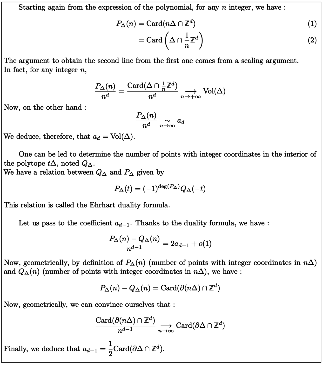
We are able to give a geometric interpretation as well as the explicit expression of some coefficients of the Ehrhart polynomial

Indeed, the dominant coefficient a_d is equal to the volume of ∆ and the second coefficient a_d−1 is related to the number of points with integer coordinates on the boundary:

Also, the constant coefficient is equal to 1, since if we evaluate the polynomial at 0, we find the number of points in 0∆ which is none other than the origin. With all these information, we can explicitly determine the expression of the Ehrhart polynomial of two-dimensional polygon ∆:

Although the Ehrhart polynomials still raises a lot of mathematical questions, it has recently found applications in computer science.

In computer science, it sometimes happens that even simple programs take a long time to be executed. This can be due to a problem of storage and access to the information during the execution, in particular when passing through nested loops. To alleviate this problem, we can use ranking Ehrhart polynomials and their inverses.

Ranking Ehrhart polynomials are generalizations of Ehrhart polynomials : to any polytope ∆, we associate the polynomial P_∆ with d variables such that P_∆(i₁, · · · , i_d) equals the number of points with integer coordinates contained in ∆ that are smaller than (i₁, · · · , i_d) for the lexicographic order. For each points (i₁, · · · , i_d), P_∆(i₁, · · · , i_d) is actually a sum of Ehrahrt polynomials associated to different polytopes. In particular, P_∆(i₁, · · · , i_d) is the rank of i₁, · · · , i_d in ∆ when sorting elements in lexicographic order.

How can it be used ? Consider the following piece of program:

where a, b and c represent N × N arrays. In the computer memory, the values of the matrices a, b and c are stored line by line. However, the program does not access them in this order and then spends a lot of time. It would be better to store the data in the order they are visited by the algorithm. To do that, we consider the following polytope:

The integer points of ∆ correspond to all the triplets present in the loops. Then arrays a, b and c can be next stored using the rank of the elements given by the Ehrhart polynomial. This can be further used to rewrite the loops and optimize the parallell execution of the program on several processors.

In conclusion, Ehrahrt polynomials have some very beautiful mathematical properties but still hold some mysteries. Nevertheless, this does not prevent us from using them in very concrete problems in computer science. Ehrhart polynomials have been a very useful discovery nowadays to reduce the computation time of algorithms.

ANNEX

02/12/2021 - Optimal Transport and astrophysics

This article was written by Claire SCHNOEBELEN and Nicolas STUTZ, based on the presentations given by Nicolas JUILLET and Bruno LEVY on December 2nd, 2021.

Discrete-discrete (left) and discrete-continuous optimal transport (Source: [1])

The theory of optimal transport began at the end of the 1770s. The mathematician Gaspard Monge formalized the problem of "cut and fill". Historically, one sought to move a pile of earth from an initial region of space (called excavation), possibly modifying its shape, to a final region (called embankment) in an optimal way. This is in fact a displacement problem that describes more general situations, where the mass to be transported can be considered as a gas, a liquid, a cloud of points, or even grey levels in the context of image processing.

The so-called matching problems are natural examples of transport problems, and we will explain one of them. Let us give an integer n and consider n mines x₁ , . . . , x_n from which an ore is extracted, as well as n factories y₁, . . . , y_nusing this ore as raw material. We try to associate to each mine x_ia plant y_j in order to minimize the total transportation cost. To model the problem, let us note c(x_i,y_j) = c_ij the cost of moving an ore from a mine x_i to a plant y_j. The solution of the problem then reduces to finding a permutation σ_optsuch as

that is solution of the following minimization problem:

Note that the problem and its potential solutions depend on the chosen cost function. In our example, we could identify the mines x_i and the factories y_jwith points of a Euclidean space and consider cost functions of type "distance", i.e.

A remarkable property of the theory of discrete transport appears in this context as a consequence of the trian- gular inequality : the optimal transport paths do not intersect. Moreover, we can reformulate the above problem. Formally, we look for an application T_opt solution of the minimization problem:

We can generalize the previous problem as follows. We still consider n plants to be delivered but there are now m ≠ n mines producing the ore. With the previous modeling, if m < n, the optimal transport function will not be surjective and some plants will not be delivered.

Kantorovich’s formulation of the transportation problem takes this case into account: it involves distributing the ore from each mine to several plants. More precisely, we assign masses p₁,...,p_m (resp. q₁,...,q_n) to the mines x₁,...,x_m (resp. to the plants y₁,...,y_n) by imposing that there is as much ore at the source as at the demand

The problem then becomes to assign masses to the m×n transport routes, i.e. to find a matrix, called "transport plan":

(where M_ij ≥ 0 represents the mass transported from x_ito y_j) in the solution of the minimization problem:

by respecting the conservation of the outgoing and incoming masses:

So far we have only dealt with discrete transport problems. There is a more general formalism in which the displaced mass is represented using probability measures, which can be discrete or continuous. The Kantorovich transport problem in its general formulation then takes the following form: considering two probability measures

(thinking of the first as excavation, the second as embankment) , we look for π_opta measure (a transport plane) solution of the minimization problem

with the following margin equations (mass conservation conditions):

The algorithmic aspect of the optimal transport problem has been the source of numerous works since those of the mathematician Leonid Kantorovich in the middle of the 20th century. In astrophysics, the theory of optimal transport is notably used to reconstitute the great movements of matter in the early universe. More precisely, it is a question of finding the transport process which, from a uniform spatial distribution at the beginning of the Universe, has led to the present structures.

In a classical approach, the present matter clusters are represented by a set of points in space Y = (y_j)_j∈J, distributed according to the present observations. In the same way, the matter at the beginning of the Universe is represented by a set X = (x_i)_i∈Iof points uniformly distributed in space. Now, we have to find the application T ∶ X → Y which associates to each point of X the point of Y on which the corresponding matter was sent with time.

To give a satisfactory account of the transport process, X would have to have a large number of points. But finding T is in fact the same as finding the corresponding I → J application and is therefore a matter of combinatorics. Therefore, the algorithms exploiting a discrete-discrete modeling of this problem are of quadratic complexity. Thus, it quickly becomes numerically very expensive to solve it with X of large size.

One way to avoid this problem is to consider the "limiting case" in which X contains all the points in space. The reformulated problem is one of semi-discrete transport, in which the initial distribution ρ(x) is a uniform density and the arrival distribution

is discrete. In this new problem, the cost minimized by the transport function T is given by:

Reconstruction of the initial cosmological density field (Source: [1])

where x represents a mass element of the space V in R³ and ρ the initial density. It is then possible to show that in this case, portions of the space, called Laguerre cells, are sent to points.

In order to determine these Laguerre cells associated with the optimal transport, the previous problem is reformulated in its dual form, as a maximization problem. This problem can then be solved efficiently with a Newton algorithm. Finally, the numerical reconstruction of the transport of matter in the Universe can be done in O(N log N ) where N denotes the cardinal of the set Y, which is a considerable progress compared to combinatorial algorithms.
We see here that a change of point of view reduces the initial discrete problem to an a priori more complex case because it involves a continuous space, but in fact allows to treat it numerically in a more efficient way.

References:
[1] Lévy, B., Mohayaee, R. & von Hausegger, S. (2021). A fast semi-discrete optimal transport algorithm for a unique reconstruction of the early Universe. Monthly Notices of the Royal Astronomy Society.

18/11/2021 - Wavelets and astrophysics

This article was written by Robin RIEGEL and Claire SCHNOEBELEN, based on the presentations given by Erwan ALLYS and Philippe HELLUY on November 18th, 2021.

The analysis of an image, represented by a matrix coding the gray level of each pixel, consists in a series of mathematical operations highlighting the important components useful for the future analyses and treatments. In that regard, the wavelet method is a remarkably efficient tool. Through successive convolutions of the signal with maps called "wavelets", this method manage to obtain information relating to the amplitude and phases at different scales, as well as interactions between scales. For a signal composed of 2^J points, the method consists in computing J + 1 series of 2^jcoefficients, noted s_j,k for j going from 0 to J and k going from 0 to 2^j − 1. These coefficients are obtained by convolving the signal with maps φ_j,k, called "daughter wavelets", all obtained by translation and dilation of a single map φ, called "mother wavelet".

Different mother wavelets can be used. The Daubechies wavelets are for example used for image compression. In this case, the coefficients are in practice obtained by recurrence, starting from the J series, made up of the points of the signal : the coefficients of the j series are obtained by performing a linear combination of neighboring coefficients in the j+1 series. Another linear combination of the same coefficients gives the "details" d_j,k. The last step thus produces a single coefficient s₀ and 2^J−1 details. Unlike Haar’s method in which the details cancel only when the signal is locally constant, the linear combinations involved in Daubechies’ method are chosen so that the details also cancel when the signal is locally linear. The original signal can be fully reconstructed from the s₀coefficient and the non-zero details computed in the last step. Moreover, the removal of the coefficients close to zero results in a minimal loss of information and is therefore a very efficient method for signal compression. This algorithm, applied to the lines then to the columns of pixels of the images, is in particular used to compress them in the storage format JPEG2000.

Another mother wavelet, the one we will discuss in the following, is the Morlet wavelet, obtained by multiplying a Gaussian by a complex exponential:

with n a vector of the plane and σ > 0 the scale parameter of the Gaussian. The convolution with one of these wavelets acts as a band-pass filter on the planar signal which thus allows to quantify the variations in the n direction at the scale 1/σ.

This type of wavelet can thus be used to highlight the interactions between scales in a given signal. It is therefore of particular interest in the analysis of astrophysical images, especially in the analysis of the structures of the interstellar medium (ISM). Indeed, on the images we have, the latter does not have the appearance of a Gaussian field, entirely characterized by its power spectrum and without interactions between scales. On the contrary, the constructive interference between the different scales induces complex structures that we would like to analyze. A very efficient technique to study images is to use neural networks but it is difficult to implement in our case, because of the limited number of data available. Thanks to the wavelet method, it is however possible to imitate these treatments in a totally controlled way and from a single image.

This involves calculating three series of coefficients, the Wavelet Scattering Transform, by convolving the image I with the wavelets discussed in the previous paragraph:

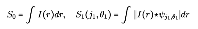
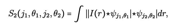
where j₁,j₂and θ₁,θ₂ are respectively the scales and the directions of the considered wavelets. The first coefficient accounts for the average value of the image I and those of the second series allow to isolate the components of the image related to a direction and a given scale. The third set of coefficients accounts for interactions between scales and directions. The key point in these formulas is the use of the modulus of the images which introduces a non-linearity. Just as in neural networks, this non-linear operation is an integral part of the process in that it reveals the interferences between the different scales.

Computation of Phase Harmonic Wavelet moments (Source: [1])

Another non-linear operation that one can introduce is the phase harmonic. This operation allows to build statistics called Wavelet Phase Harmonics (WPH) in four steps. One starts by filtering an image at two different scales and then performs a phase harmonic which modifies the phase of one of the two images to obtain two images of the same phase now correlated. It is now of interest to compute the different covariance moments of these images and from them build the WPH statistics. The calculated moments quantify the interactions between two given scales, the WPH statistics of an image characterizes its structure. Knowing these statistics, it is then possible to generate a large quantity of images with the same properties. We thus obtain a generative model.

A major application of this generative model is the study of the Cosmic Microwave Background (CMB) which allows us to learn more about the formation of our universe and its large structures. Indeed, it is difficult to separate the CMB from structures such as the Milky Way or stars. The WPH statistics can then simulate a large number of images of these foregrounds from a single other image. The latter having a non-Gaussian structure, unlike the CMB, one can train a neural network to perform the separation and thus obtain data useful for the study of the stellar background.

The wavelet method is thus a central tool for the multiscale analysis of images. Particularly adapted for image compression, it requires extensions to better account for interferences between scales and could thus help to better observe the cosmological background for a better understanding of the evolution of the Universe.

References:

[1] Allys, E., Marchand, T., Cardoso, J. F., Villaescusa-Navarro, F., Ho, S., & Mallat, S. (2020). New interpretable statistics for large-scale structure analysis and generation. Physical Review D, 102(10), 103506.

04/11/2021 - Discrete geometry for images and point clouds

This article was written by Victor LE GUILLOUX and Lucas PALAZOLLO, based on the presentations given by Etienne BAUDRIER and Quentin MERIGOT on November 4th, 2021.

A shape and its digitization (Source: [1])

Discrete geometry makes it possible to develop various mathematical tools to characterise the geometry and topology of objects contained in an image, i.e. the shape of a subset of pixels or voxels in an image. These tools are used, in particular, in biomedical imaging and materials science. From an image partition or even a point cloud, we try to obtain an efficient model thanks to numerous estimators to calculate lengths or to model precisely its curves and edges.

In order to calculate discrete geometric quantities of an object such as its volume, length or curvature, it is essential to use estimators that converge to the continuous geometric quantities we are seeking as the resolution of the image increases. This type of convergence is called multigrid convergence. Let us denote by h the discretization step of the grid, i.e. the size of the pixels, Ɛ̃ the discrete estimator, Ɛ the continuous geometrical characteristic and F a family of shapes. Then the convergence of the estimator can be written :

Consider the example of the perimeter estimator. First, we can think of counting the number of elementary moves : we count the number of horizontal and vertical moves by following the pixels at the edge of the studied shape. However, we end up calculating the perimeter of the rectangle in which our shape is inscribed, which does not make it a reliable estimator at all. More generally, it can be shown that estimators based on elementary moves are doomed to failure because they would only converge for a countable set of segments.

Detection of edges in a cloud of points (Source: [2])

One solution is to estimate the length by polygonalization, i.e. by discretizing the curve by line segments. The line segments form a polygon whose perimeter is easy to calculate. To solve this problem, an algorithm is used to detect whether the pixels belong to the same discretised line segment. Thus, the set of largest line segments is sought. It can be shown that this estimator converges in O(h^1/2). In the previous algorithm, the maximum line segments are used as a pattern, but it is possible to use other methods by changing the patterns.

When the shape is obtained using measurements, it is no longer defined as a connected subset of pixels but as a point cloud. Specific methods have therefore been proposed as the so-called distance-based geometric inference methods. Given an object K, one can for example retrieve information about its curvature by using a tubular neighborhood of K, i.e. by considering all points located at a smaller distance than a given distance (the scale parameter) from the object K in question. If r ≥ 0 denotes the scale parameter, let us denote by K^r the tubular neighborhood of K for the parameter r. The first result on these tubular neighborhoods is Weyl’s Theorem, stating that the d-dimensional volume of the neighborhood K^r is a polynomial function of degree d on a certain interval, whose size is specified by Federer’s Theorem. More precisely, Federer’s Theorem describes the boundary measure of K. This measure gives a weight to any subset B of K as follows :

where H^d denotes the d-dimensional volume and p_K denotes the projection onto K. This measure contains the information of the importance of the local curvature of K in B because it gives a higher weight to subsets of strong curvature. Federer’s Theorem then states that there are signed measures Φ0, . . . , Φd such that for a small enough r :

and it is these signed measures that contain the information about the local curvature of K, in particular about the possible edges of K.

The question then arises as how to calculate, in practice, the boundary measure of an object. To compute it, we use a Monte-Carlo-type method. This method consists in choosing a large number of points in the neighborhood of the object, and using them to compute a discrete estimator of the boundary measure : each point is somehow projected on the edge of the object and gives a positive weight to the projection location. The larger the number of sample points is, the higher will be the probability of obtaining a maesure that approaches well the boundary measure.

These examples show the diversity of methods used in the discrete estimation of continuous objects in order to retreive their geometrical and topological properties. Discrete geometry provides robust and efficient tools. Moreover, extensive mathematical studies are needed to determine the accuracy of the different estimators and to ensure their relevance to the problems considered.

References:

[1] Lachaud, J.O., & Thibert, B. (2016). Properties of Gauss digitized shapes and digital surface integration. Journal of Mathematical Imaging and Vision, 54(2), 162-180.

[2] Mérigot, Q., Ovsjanikov, M., & Guibas, L.J. (2010). Voronoi-based curvature and feature estimation from point clouds. IEEE Transactions on Visualization and Computer Graphics, 17(6), 743-756.

21/10/2021 - Lung ventilation modelling and high performance computing

This article was written by Nina KESSLER and Samuel STEPHAN, based on the presentations given by Céline GRANDMONT and Hugo LECLERC on October 21st, 2021.

The lungs allow the oxygenation of the blood and the removal of carbon dioxide produced by the body. To achieve this, the lung tissue has a special tree-like structure that allows air to travel from the trachea to the alveoli in the lungs. This tree has an average of 23 generations of increasingly smaller bronchi for a human lung. The fact that we can breathe effortlessly at rest is due to the pressure difference between the alveoli and the surrounding air, as well as the elasticity of the tissues. However, certain pathologies can interfere with this process, such as asthma, which causes the diameter of the bronchial tubes to decrease, reducing breathing capacity. Dust particles or pollution can also affect breathing. In order to better understand the behaviour of the pulmonary system and to provide analysis tools in pathological cases, mathematical modelling has been proposed.

Bronchial tree modelling with a dyadic tree of pipes. (Source: [1])

The lungs can be modelled as a tree of N = 23 generations of bronchi, each branch of which represents a bronchus with, in the last generation, alveoli represented by separate masses of springs. To a first approximation, the airflow in each bronchus is only characterised by one parameter, the resistance R. The flow rate Q is then directly related to the pressure difference at the entrance and exit of the bronchus ∆P by the relation ∆P = RQ. Air transport can therefore be modelled mathematically by means of a tree of 2N resistances. The resistance associated with the i-th generation bronchi is of the form R_i = R_i−1/β³ = R₀/β³ⁱwith β = 0.85. Therefore, at the level of the alveoli, since the flow is equal to Q₂₃ = Q₀/2²³, the total pressure difference is equal to R₂₃Q₂₃ = R₀Q₀/(2β³)²³ = (1.63/2)²³R₀Q₀. It is then possible to determine the movement of the cells under the effect of the pressure. The position u_i(t) of the i-th cell satisfies the differential equation :

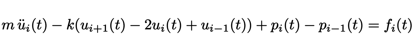
where the pressure term

takes into account the coupling through the bronchial tree. It can be implemented numerically and compared with experimental data from dynamic lung imaging. These data allow us to determine the parameters of the model, test its limitations and then improve it. Some of the limitations are due to the conditions at the edges, i.e. the way the bronchial tree and the air at its entrance interact. But others are practical, as we will see later, due to the computational cost of the numerical simulations.

The previous model was used to study respiratory treatments based on Heliox. Heliox is a mixture of helium and oxygen that could make it easier for people with lung diseases to breathe. It is a less dense gas, but more viscous than air. The resistance within the bronchial tree is globally reduced, and the result is that Heliox has a laminar regime when it passes through a pipe with a low flow. This gas therefore reduces the effort required to breathe. However, when the gas flow rate becomes high, the benefits of the product are considerably reduced due to its viscosity. By providing a description of the overall dynamics of ventilation, the model allows a more detailed analysis of its impact on breathing and helps to determine when it is actually beneficial to use it.

The application of the models described above on concrete cases requires a more precise description of the flow in the first bronchi and therefore the acquisition of data on patients. This can be done with the help of tomography, which allows a 3D image to be reconstructed from a 2D image sequence. A segmentation algorithm must then be applied to create a volume mesh of the bronchial tree. However, the basic algorithms for reconstructing a CT image are not suitable. Indeed, the movements of the organs in the thoracic wall make the data acquisition noisy. A recently proposed segmentation method consists of starting with a small sphere contained in a zone of the tree and then progressively enlarging it while minimising its total surface area at each moment.

For this problem, but also for many others in mathematics, the quantity of data to be manipulated can be very large, thus generating algorithm execution times that we would like to avoid. To reduce these execution times, it is necessary to manage more finely the calculations carried out by the processors and the accesses to the RAM memory. Optimal use of a processor involves parallelizing the calculations it is given to perform. It may therefore be useful to vectorise calculations, i.e. to allow the processor to perform simultaneous operations on neighbouring data. It is also sometimes necessary to redefine the numerical methods themselves to take advantage of the new performance of the calculation tools. For example, it is possible to create very precise numerical methods using symbolic computation. These methods potentially require more computation but less communication with memory.

The example of lung tissue is a perfect illustration of the different steps required to study complex physiological phenomena. Even with a lot of approximations on mechanics and geometry, this approach makes it possible to establish simplified models that make it possible to explain certain data and then eventually orient certain therapeutic studies. This work therefore involves multiple skills ranging from model analysis to a thorough mastery of computer tools to accelerate the numerical simulations of the models.

References:

[1] Grandmont, C., Maury, B., & Meunier, N. (2006). A viscoelastic model with non-local damping application to the human lungs. ESAIM: Mathematical Modelling and Numerical Analysis, 40(1), 201-224.

07/10/2021 - Turbulence, aeronautics and fluid-particle dynamics

This article was written by Raphaël COLIN and Thomas LUTZ-WENTZEL, based on the presentations given by Abderahmane MAROUF and Markus UHLMANN on October 7th, 2021.

Turbulence simulation near an aircraft wing using RANS method (Source: [1])

The experiments of Osborne Reynolds (1883) have shown the existence of two regimes of fluid flow : laminar and turbulent. By running a fluid through a cylindrical pipe at a controlled rate, he noticed a change in the behavior of the flow as the flow rate increased. The fluid goes from a regular state to a disordered state, which correspond respectively to the laminar and turbulent regimes.

The phenomenon of turbulence refers to the state of a liquid or a gas in which the velocity presents a vortical character at any point. These vortices, present at different length scales, up to the microscopic scale, see their size, their orientation and their localization change constantly in time.

Reynolds introduced, following his experiments, the Reynolds number :

where ρ is the density of the fluid, U its characteristic velocity, μ its viscosity coefficient and D the reference length (for example the diameter of the cylinder in the Reynolds experiment). This number characterizes the behavior of the fluid in a given domain. A large value of Re is associated with a turbulent behavior.

The Navier-Stokes equations describe the behavior of incompressible fluids. They are written :

The numerical solution of these equations in the case of a turbulent fluid is difficult. Indeed, to do so, one must discretize the space using a spatial mesh. One then obtains cells (small volumes) in which the velocity and pressure are constant and evolve over time. A good approximation requires to control what happens inside these cells : we want the fluid to be regular. The presence of vortices at the microscopic scale leads us to consider very thin meshes, which considerably increases the computational cost.

Various methods are available for numerical resolution, for instance DNS (direct numerical simulation) and RANS (Reynolds Averaged Navier-Stokes).

One the one hand, DNS is the more precise of the two, it consists in solving directly the Navier-Stokes equations by using a mesh fine enough to capture the smallest vortex structures. It has the disadvantage of being computationally expensive, which can make it unusable in practice.

The RANS (Reynolds Averaged Navier Stokes) method, on the other hand, is based on a local statistical description of the velocity field. To do this, the velocity in each cell is decomposed as the sum of a mean velocity and a disturbance term :

By injecting it into the equations and after simplifications, we obtain the following equation :

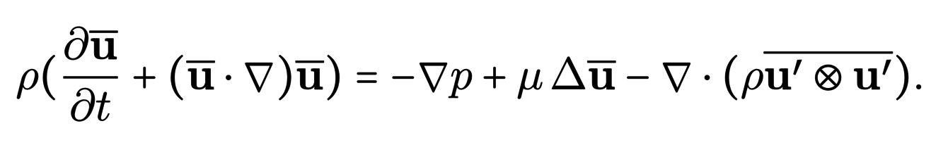
The last term of this equation, called the Reynolds stress tensor, encodes the effect of the fluctuations around the mean velocity and RANS methods actually proposed to model this term using Eddy viscosity assumptions. The obtained models allow the use of coarser meshes that will capture the majority of vortex structures. This method is less accurate than DNS but has a more reasonable computational cost.

These numerical methods are used in many applications. For example, in aeronautics, the boundary layer phenomenon gives rise to turbulent airflow on the surface of aircraft wings. This can lead to a decrease in aerodynamic performance and even to the breakage of the wing via the resonance phenomenon. Bio-morphing techniques aim to develop wings that are adaptable over time, in order to reduce the impact of turbulence on them. For instance, through a controlled variation of the temperature of the materials constituting the wing, we can modify their rigidity during the flight. This allows their deformation into a shape adapted to the flight phase considered.

It is also interesting to study the behavior of particles in turbulent fluids, since this type of system is omnipresent in nature (clouds, sediment transport, etc.) or in industrial systems (solar furnaces). Fluids and particles interact in a complex way since turbulence influences the dynamics of particles and particles can themselves modify the turbulent properties of the fluid.

Particle dynamics in turbulent flows (Source: [2])

The spatial distribution of the particles is for example modified by the centrifugal force due to the vortex structures of the turbulent fluid, but also by the wake effect (the particles that follow others are less slowed down by the fluid, which has the effect of grouping the particles). Turbulent fluids also have an influence on the settling velocity of the particles (velocity reached when the fluid resistance reduces the acceleration of the particle to zero, its velocity does not evolve any more), for example, some particles will be attracted by some parts of the vortex structures, which has an effect on their settling velocity. The effect of particles on turbulence is not well understood, and requires the use of different models for the particles and the fluid, which must then be successfully combined. The particles can reduce or amplify the turbulent behavior of the fluid (increase the speed of the vortices or dissipate them).

To simulate such fluid-particle systems, there are several interactions to be computed : the effects of the fluid on the particles and of the particles on the fluid, and the particle-particle interactions. For the fluid-particle interactions, one can use the submerged boundary method, where in addition to the mesh which is a sampling of the space, the surface of the particles is sampled at different points on which the forces that apply are computed. The motion of the particles can be calculated with a discrete version of Newton’s equations. Other methods also exist, in particular methods that use an adaptive space mesh (finer around the particles and coarser elsewhere), to reduce the computational cost. The computation of interactions between particles require more classical methods of collision detection and application of forces.

We have seen that DNS methods are very expensive in terms of computational resources, and it is appropriate to focus on the performance of such simulations. It is possible to divide the regular grid on which we work into a number of subdomains, each of which can be associated with a processor, in order to process the calculations in parallel. Thus, new problems can arise, for example, on the treatment of particles when they travel from one subdomain to another, and the balancing of the computational load (indeed, what to do if the majority of the particles are in a single subdomain ?).

Turbulence is a phenomenon that occurs in many fields such as aeronautics or solar oven design. The development of small-scale vortex forms requires the development of efficient numerical methods with optimized computational capacities or using simplified models.

References:
[1] Marouf, A., Simiriotis, N., Tô, J.-B., Rouchon, J.-F., Braza, M., Hoarau, Y. (2019). Morphing for smart wing design through RNAS/LES methods . ERCOFTAC Bulletin.

[2] Chouippe, A., Uhlmann, M. (2019). On the influence of forced homogeneous-isotropic turbulence on the settling and clustering of finite-size particles. Acta Mechanica, 230(2), 387-412.

23/09/2021 - Symplectic geometry and astrophysics

This article was written by Robin RIEGEL and Nicolas STUTZ, based on the presentations given by Rodrigo IBATA and Alexandru OANCEA on September 23rd, 2021.

Stellar streams obtained from the Gaia satellite (Source: [1])

Dark matter makes up about 25% of the Universe but is still very mysterious. The standard model of cosmology called ΛCDM provides a theory to account for the interactions of dark matter with the structures of the Universe.

In order to validate this model, one possibility is to study the residues of low-mass star clusters orbiting the Milky Way, called stellar streams, interacting with dark matter and whose trajectories have been recorded by the Gaia satellite. But this is very difficult. Indeed, the ΛCDM model predicts the accelerations of these stars but it is impossible to measure these accelerations in a suitable time. It would take thousands or even millions of years for such structures with our current instruments.

Another approach is then considered, and we will see that the tools of symplectic geometry play an integral part.

Instead of using the data to validate a theoretical model, astrophysicists try to build a model from the data. More precisely, it is a question of determining the Hamiltonian function H(q,p), or energy of the system, function of the positions q = (q1,...,qN) and impulses p = (p1,...,pN). The associated Hamiltonian dyamic is the following differential system:

As it is, this system is too complicated to learn H from the data. However, the tools of symplectic geometry allow us to simplify the study of this system by expressing it in new coordinates.The goal is to find coordinates (P(p,q),Q(p,q)) allowing to obtain a simpler system to solve and giving more information about the system. The flows of this Hamiltonian system preserve the symplectic 2-form and thus some associated properties such as the volume for example. Thus, coordinate changes of the form (P, Q) = φ(p, q) where φ is a flow of the system are preferred transformations. Such a coordinate change is called a canonical transformation.

The natural coordinates to look for are the action-angle coordinates (θ(p,q),J(p,q)) solutions of a Hamiltonian system :

Sketch of the method used in [2] for learning action-angle coordinates

Indeed, for this coordinate system, the Hamiltonian K(θ,J) then does not depend on θ and the integration is easier. Moreover, J is constant along the trajectories of each star.

This coordinate system gives a lot of information: it allows to clearly identify the considered objects and finally to deduce the acceleration field.

How then to find these action-angle coordinates from the data? Jacobi introduced about 200 years ago the so-called generating functions S(q, P ) of a canonical transformation (P, Q) = φ(p, q).

This function verifies the relations

These conditions result from the fact that the symplectic form cancels on the set

This generating function thus ensures that the coordinate change preserves the symplectic structure. To determine the coordinates (θ,J) from the data, it is possible to use a neural network-based deep learning method that computes the generating function by imposing that J is invariant on each trajectory.

Thus, starting from the observations of stellar streams and studying the Hamiltonian system, we can determine coordinates (θ,J) and find the Hamiltonian of this system. The latter contains all the physics of the system and in particular the effect of dark matter on the dynamics of stars. This is why the study of stellar streams is very promising to probe the dark matter by confronting the calculated acceleration fields with those predicted by the ΛCDM model.

References:
[1] Ibata, R., Malhan, K., Martin, N., Aubert, D., Famaey, B., Bianchini, P., Monari, G., Siebert, A., Thomas, G.F., Bellazzini, M., Bonifacio, P., Renaud, F. (2021). Charting the Galactic Acceleration Field. I. A Search for Stellar Streams with Gaia DR2 and EDR3 with Follow-up from ESPaDOnS and UVES. The Astrophysical Journal, 914(2), 123.

[2] Ibata, R., Diakogiannis, F. I., Famaey, B., & Monari, G. (2021). The ACTIONFINDER: An unsupervised deep learning algorithm for calculating actions and the acceleration field from a set of orbit segments. The Astrophysical Journal, 915(1), 5.

09/09/2021 - Discrete differential geometry

This article was written by Philippe FUCHS and Claire SCHNOEBELEN, based on the presentations given by Mathieu DESBRUN and Franck HETROY-WHEELER on September 9th, 2021.

It is frequent that a lifelike object is modelized by a surface for the needs of animations or 3D simulations. In order to be manipulated by computers, whose calculation and storage capacities are limited, the contours of this object are approximated by a finite number of juxtaposed polygons, the whole of which is called a ”mesh”. It is this discrete representation of the object’s surface that is then used numerically.

Mean curvature on a horse mesh (Source: [1])

To analyse and manipulate these surfaces, it is interesting to approach them from the point of view of differential geometry. This subject allows, especially through the concepts of curvatures, to characterize the regular surfaces. However, in order to use these tools on our polygonal surfaces, it is necessary to extend their definitions beforehand. Let us consider for example the curvature, a central notion in the study of surfaces. As it is defined on a smooth surface, it has no meaning on a piecewise planar surface. As we will see later, it is however possible to redefine the notions of curvature using the Gauss-Bonnet formula and the discrete Laplace-Beltrami operator.

Let us now see how curvature is defined for a regular surface. On such a surface, each point x is contained in a neighbourhood V parametrized by a certain smooth application X with values of an open U of the plane in V. The set of local parametrizations X describes a folding of the surface in R³. The first derivatives of X determine the so-called first fundamental form, a quadratic form from which we define a distance on the surface. The second derivatives of X determine the shape operator of the surface, from which the different notions of curvature are defined. The Gaussian curvature and the mean curvature in x are thus defined as being respectively the determinant and half of the trace of this operator.

Of these two notions of curvature, only one is independent of the folding: the mean curvature. The Gaussian curvature can in fact be expressed as a function of the coefficients of the first fundamental form and its derivatives which, unlike the shape operator, do not depend on the folding of the surface in R³. For this reason, the Gaussian curvature is said to be intrinsic and the mean curvature is said to be extrinsic. In general, a quantity is extrinsic if it depends on the folding of the surface in R³, in other words if it is necessary to consider the position of the surface in space to measure it. On the contrary, the intrinsic quantities are those which can be defined on the surface as a set with its own properties, without having recourse to the surrounding space, and which do not depend on the way the surface is observed from the outside. The plane and the cylinder, for example, have the same first fundamental shape, and thus the same Gaussian curvature, but not the same mean curvature. This illustrates the fact that they are two locally isometric surfaces plunged differently in R³.

Let us now see how to define the curvature on our polygonal surfaces. It is not possible to define a shape operator on them as it was done on regular surfaces. To extend the two previous notions of curvature, it is necessary to approach them differently. We know for example that the Gaussian curvature K is involved in the Gauss-Bonnet formula:

where χ(S) represents the Euler characteristic of the surface and the ε_i the exterior angles of the edge of the Ω domain. By choosing a neighbourhood Ω of x in our polygonal surface, we can define the Gaussian curvature at x as

where A is the area ofΩ. In the same way, we can extend the definition of mean curvature by starting from the following equality:

where ∆ is the Laplace operator on the surface. It is possible to give an equivalent to this operator in the case of polygonal surfaces: the discrete Laplace-Beltrami operator. The previous formula, applied to this new operator, allows us to define the average curvature of our surface in x.

The process which consists in exploiting some properties of a notion used in differential geometry in order to propose a definition in the discrete case can be used for other generalizations. For example, to smoothen the noise of a surface scan, we would like to apply a method similar to the nonlinear diffusion used on regular surfaces, given by

where n is a normal vector to the surface. However, the previous equation cannot be immediately applied to polygonal surfaces. Returning to the origin of this equation, we see that the motion u of the surface that it describes is in fact the one that minimizes the area the fastest. Having noticed this, it is easy, by using the gradient of the area, to develop a method for denoising polygonal surfaces which, when the mesh becomes finer and finer and tends towards a regular surface, amounts to applying the nonlinear diffusion that we started with.

Field lines on a surface with singularities at red and green points (Source: [2])

The extension of the concepts of differential geometry on polygonal surfaces has many other practical applications. For example, let us suppose that we want to draw the coat of an animal in an animated film. We model the animal in question by a polygonal surface and its coat by a vector field on this surface. In order to render it realistically, we would like to create a smooth field almost everywhere and determine the singularities in advance.

The most common way to do this is to exploit parallel transport. This notion, first defined on regular surfaces, can easily be generalized to piecewise planar surfaces. On a plane, the parallel transport related to the Levi-Civita connection takes the very simple form of a translation. To define it on the whole surface, we just have to determine the way to transport a vector v from a face P to one of its neighbours P′. To do this, we consider the two faces as two pieces of a plane that we have folded. Let’s unfold it for a moment: the two faces are now part of the same plane, on which we can transport v by translating it from one face to the other. Let’s fold back our two faces. The vector obtained after translation of v is a tangent vector to P′ and it is this one that we define as the parallel transport of v from P to P′.

In defining parallel transport in this way, we come up against the notion of holonomy. Consider a vertex of our polygonal surface and the set of faces attached to it. By transporting a vector from one face to another with the process described above, it is possible that the vector obtained after having made a complete turn of the vertex by passing from face to face is not collinear with the original vector. This will in fact be the case as soon as these faces are not all coplanar. In order to avoid this kind of phenomenon, we add a step to what precedes. For each pair of faces, we compose the translation on the unfolded faces with a rotation, so that the parallel transport of a vector around a vertex coincides with the origin vector. It is possible to define these rotations on the whole surface by ensuring that around almost all vertices the transport of a vector coincides with itself: the set of angles of these rotations are solutions of a large linear system. With this method, it is also possible to define in advance the vertices around which the holonomy will not be zero. By proceeding in this way, one can, from a single vector carried on all faces, construct a smooth vector field everywhere on the surface except at a few predetermined points.

The two previous examples illustrate the interest of extending the tools of differential geometry to polygonal surfaces: the application of the tools of discrete differential geometry has allowed us to build two efficient and elegant methods to solve concrete 3D imaging problems.

References:
[1] Meyer, M., Desbrun, M., Schröder, P., & Barr, A. H. (2003). Discrete differential-geometry operators for triangulated 2-manifolds. In Visualization and mathematics III (pp. 35-57). Springer, Berlin, Heidelberg.
[2] Crane, K., Desbrun, M., & Schröder, P. (2010, July). Trivial connections on discrete surfaces. In Computer Graphics Forum (Vol. 29, No. 5, pp. 1525-1533). Oxford, UK: Blackwell Publishing Ltd.